
If you have ever spent hours manually totaling up figures in a spreadsheet, you understand that Microsoft Excel is a tool that saves you time, but only when you know the right spells to cast. For many people, the basic sumif excel formula is a lifesaver. It is just wonderful for a basic sumif excel example, like if you are only trying to figure out the full sales number made by one person selling stuff. Say you need to total up sales for a certain kind of product and it also has to be sold in a particular area? That is when the simple way stops working. That is when you need to level up your game and tackle the real power of (Sumif Multiple Criteria), which often involves understanding the and or function in excel logic.
Learning to implement (Sumif Multiple Criteria) is truly essential for moving beyond basic data entry and toward actual data analysis. It involves using the far more robust SUMIFS function, and understanding the difference between excel formula and logic and Excel formula or logic. This is exactly where most folks sort of stumble and get mixed up with the and or function in excel. But honestly, once you grab hold of the simple parts of the sumifs formula, your big data reports and even those specialized excel dashboard templates you make are going to look tons neater.
The Essential Difference: SUMIF Versus SUMIFS
Before diving into the complex cases of (Sumif Multiple Criteria), we should take a brief moment to clarify a common point of confusion. The older, singular sumif excel function is still great, but it has one fundamental limitation: it can only handle one condition. If you want a basic sumif example, you would write something like
=SUMIF(A:A, “Apples”, C:C) to sum the price of all “Apples.”
That moment when you bring in a second thing you are looking for—like if you need “Apples” and also “Pears”—well, that is exactly where the usual sumif excel thing in Excel just does not work good enough. This is why the SUMIFS function even had to be made! This useful function first showed up way back in Excel 2007, and it was specially built right from the start to handle sumif multiple conditions. The core difference is more than just an “S” at the end; it is in the argument order and its inherent logic type.

The SUMIFS Formula Syntax Explained
To properly use (Sumif Multiple Criteria), you must know the sumifs formula structure. Notice how it differs from the original sumif excel format:
=SUMIFS(sum_range, criteria_range1, criteria1, [criteria_range2, criteria2], …)
The key takeaway is that the sum_range (the column you want to add up) comes first in the SUMIFS function, not last as it does in SUMIF. This bit is super important, pay attention: if the list of little boxes where all your special rules are living doesn’t look exactly the same size and shape as the other list of numbers you’re trying to mush together and add up, well, the SUMIFS thing just gets all grumpy. It’ll just cough up a great, big, useless error message right in your face. Whenever you are busy dealing with a formula that needs SumIf multiple conditions, if the answer comes back as zero but you think it should not, the very first thing you usually ought to check is if all those lists of cells are exactly the right length.
Implementing the AND Logic: The Default for (Sumif Multiple Criteria)
The easiest, most direct way to get a total based on (Sumif Multiple Criteria) is when you use the \mathbf{AND} way of thinking. If you want the total sales of “Laptop” and the quantity sold is “>100”, both things must be true for the sale to be included. That is the essence of the excel formula and logic.
The excellent news is that the standard sumifs formula handles this excel formula and requirement automatically. For a powerful sumif example using the SUMIFS function, suppose we want to total the amount of “Product X” sold by the “East” region in the month of December. This is three distinct criteria, which means we are using (Sumif Multiple Criteria) with AND logic:
=SUMIFS(Sales_Amount, Product_Column, “Product X”, Region_Column, “East”, Date_Column, “>=12/1/2025”)
So, in that exact spot, the sumif excel \mathbf{SUMIFS} thing will zoom in first to look for whatever says “Product X.” Then it has to double-check if that same row is also sitting in the “East” area, and last of all, it really has to make certain the date is tucked neatly inside the month of December. That is the perfect demonstration of the baked-in excel formula and functionality of the sumifs formula. You can add up to 127 of these criteria pairs, which allows for extremely detailed data segmentation when creating advanced reports or informative excel dashboard templates.

Using Comparison Operators in (Sumif Multiple Criteria)
A great aspect of the SUMIFS function is its flexibility with conditions beyond simple text. You can use standard comparison operators (like >, <, >=, <=, <>) to define ranges.
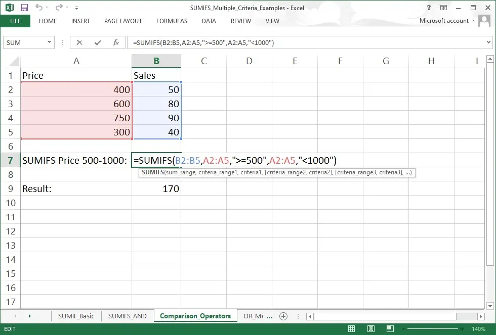
For instance, to find sales of items costing more than $500 but less than $1000, you use (Sumif Multiple Criteria) on the same column twice, once for the lower limit and once for the upper limit:
=SUMIFS(Sales_Amount, Price_Column, “>=500”, Price_Column, “<1000”)
Just remember this: when you’re using those little math symbols like > or < in the SUMIFS function, you absolutely have to wrap both the symbol and the number up inside quotation marks. It’s just the way it has to be, and you can see how it works in this super strong sumif example here. When you combine them with cell references or other functions, you must use the ampersand (\&) to concatenate the operator, a common element of the robust sumifs formula. This excel formula and technique is vital for properly applying sumif multiple conditions to date ranges, which is a frequent requirement in financial reporting for excel dashboard templates.
Implementing the OR Logic: When Any Condition Will Do
Here is the part of (Sumif Multiple Criteria) that requires clever workarounds because the SUMIFS function is not naturally designed for it. OR logic means that a value should be summed if it meets Criterion A or Criterion B or Criterion C. This is the challenge of implementing the excel formula or logic efficiently.
Just for instance, picture this: we want to figure out the total amount of money we got from selling either “Apples” or “Oranges.” If you tried to use the regular sumifs formula the way you would with an excel formula and method, Excel would spit out a giant zero! Why? Well, because one single line in your spreadsheet cannot, in all sense and logic, be counted as both an “Apple” and an “Orange” at the very same moment in time. To use true and or function in excel logic with (Sumif Multiple Criteria) and the necessary excel formula or logic, we have two primary methods:
Method 1: The Simple SUMIFS + SUMIFS Approach
The easiest way to implement Excel formula or logic for (Sumif Multiple Criteria) is simply to add multiple separate SUMIFS function results together. This way of going about it is really straight-forward and it is easy to double-check everything, too. That makes it a fantastic starting point for any simple sumif example where you only have a little handful of those OR conditions to think about:
=SUMIFS(Sales, Region, “North”) + SUMIFS(Sales, Region, “South”)
This way of doing things is good for when you have sumif multiple conditions, and it is honestly simple to figure out, even for folks who do not spend all their time messing with the sumifs formula every day.

Method 2: Using the Array Constant for Scalable OR Logic
When you have many OR conditions (e.g., ten different product names or many different salespeople), writing out SUMIFS function 10 or more times is extremely tedious. The better, more scalable way to handle (Sumif Multiple Criteria) with OR logic is to combine the SUMIFS function with the SUM function and an array constant. This is a brilliant excel formula or technique that effectively mimics the and or function in excel for use in complex excel dashboard templates.
The formula looks like this:
=SUM(SUMIFS(sum_range, criteria_range, {“Crit1”, “Crit2”, “Crit3”}))
Now, here is a neat little trick: If you put those OR conditions (things like “Crit1,” or “Crit2”) inside those special curly brackets, like this \mathbf{\{\}\}, right there inside your sumifs formula in sumif excel, Excel gets tricked into doing the SUMIFS function job for each condition all by itself. What comes out of that funny business is a whole list of answers—a bunch of numbers, really, with one number for every single thing you asked it to look up. The outer SUM function then adds all those results together, successfully implementing the required and or function in excel logic. This excel formula or technique is arguably the most elegant way to solve problems involving sumif multiple conditions when you are trying to populate complex excel dashboard templates.
For instance, to find the sum of sales for “John,” “Mike,” or “Pete,” the formula demonstrating (Sumif Multiple Criteria) would be:
=SUM(SUMIFS(D2:D9, C2:C9, {“John”, “Mike”, “Pete”}))
This is a fantastic sumif example of using an array to manage sumif multiple conditions efficiently.

Final Considerations
Mastering SUMIF Multiple Criteria
Mastering (Sumif Multiple Criteria) by properly harnessing the SUMIFS function is fundamental for efficient data manipulation in Excel. It is the core function that powers all of the conditional summarization you see in professional excel dashboard templates.
You must always remember that the default logic is excel formula and, meaning all conditions must be met. For the Excel formula or logic, you must utilize one of the array constant or SUM-plus-SUMIFS workarounds, which are part of how the and or function in excel is typically implemented in complex analysis. For a simple sumif example, stick to SUMIF, but for any situation involving sumif multiple conditions or multiple criteria, always choose the sumifs formula.
It is true that the transition from a simple sumif excel model to handling full-blown (Sumif Multiple Criteria) can feel like a jump, but the syntax is logical, and the payoff is significant. Keep practicing these techniques, and you will find your data analysis capabilities, along with the quality of your excel dashboard templates, are dramatically improved. The ability to articulate complex business logic using the powerful SUMIFS function, and or function in excel, means you are no longer just manipulating data; you are deriving genuine business intelligence, and or function in excel, and that, my friend, is a sumif example worth celebrating.
The Versatility of SUMIFS in Handling Multiple Criteria
We have now seen how the sumifs formula allows us to deal with (Sumif Multiple Criteria) with great ease. The versatility of the SUMIFS function when combined with the array technique to handle Excel formula or logic makes it indispensable, so be sure to explore these methods further. Remember to check your ranges, use quotes for text and operators, and understand the core difference between excel formula and the combined and or function in excel methods. The journey to mastering (Sumif Multiple Criteria) is certainly a rewarding one, and you’re encouraged to keep practicing these steps. You will never look at a simple sumif excel tool the same way again now that you understand sumif multiple conditions, so take a moment to apply this in your next sheet. The power of the SUMIFS function is truly incredible for every complex sumif example out there, and that is why you see it in almost all professional excel dashboard templates, try building one to see the difference yourself. This is the key to managing (Sumif Multiple Criteria) effectively, so keep refining your mastery as you move forward.