
If you have ever tried to compare two columns in excel just by looking at them, you already know it is a fast track to a massive headache and a lot of blurry vision. You start looking at row ten, your eyes skip to row twelve, and suddenly your whole report is a mess.
If you want to compare two columns in excel and quickly find differences, duplicates, and unmatched data with easy step-by-step methods, you have to stop relying on your eyes and start relying on the tools to highlight matches. Whether you are dealing with two lists of email addresses, there are actually quite a few ways to tackle this. Some people love using the if function because it is direct, while others swear by excel conditional formatting because it looks nice and makes things obvious at a glance when you highlight matches.
There are many ways to handle an excel compare two lists project. You might want to highlight matches so you can see what is the same, or maybe you are hunting for the unique values that do not belong. Depending on how your data is structured, you might use the if function, rely on excel conditional formatting to highlight matches, or go for the more advanced vlookup compare two columns technique. In this guide, I am going to break down every single way you can excel compare two lists and compare two columns in excel so you never have to worry about missing a data point again.
Method 1 Using the If Function for Row by Row Comparison
This is probably the most easiest way to excel compare two lists and check two columns in Excel if your stuff is meant to match up row by row. It works really great for a quick look to see if something got changed in a list.
- First, click in a blank cell next to your first row of data.
- Type the formula using the if function like this =IF(A2=B2, “Match”, “Mismatch”).
- Press enter and then drag that little green box at the corner of the cell all the way down to the bottom of your two columns.
- Now you can see exactly where the data breaks.
When you excel compare two lists and compare two columns in excel this way, it is very easy to then filter the results. You can just filter for “Mismatch” and you have your list of errors. This is a classic move for an excel compare columns task when accuracy is the most important thing. I use the if function all the time because it does not require a lot of fancy setup to excel compare two lists.

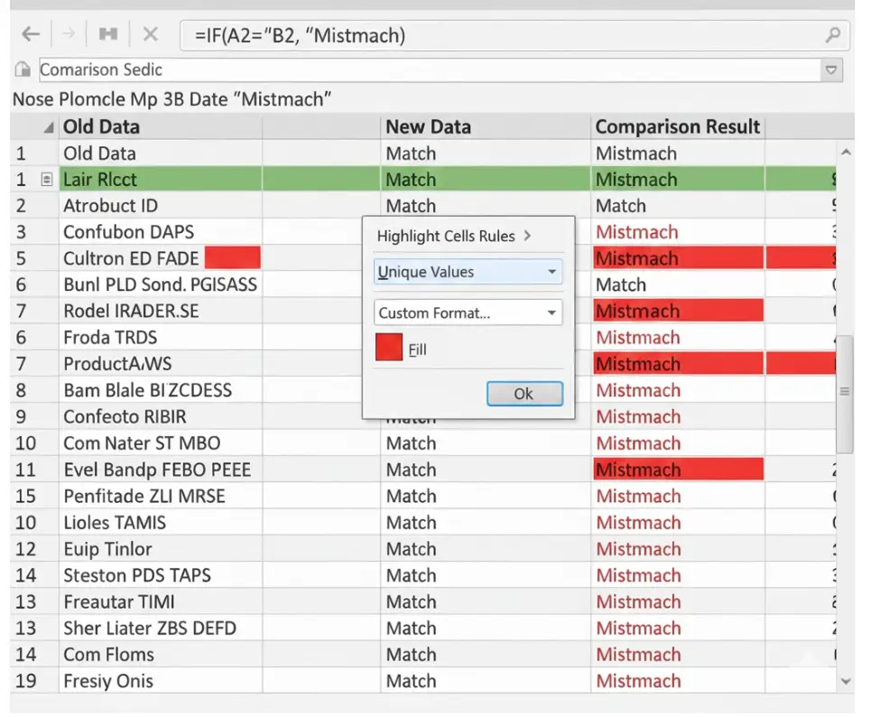
Method 2 Highlighting Differences with Excel Conditional Formatting
Sometimes you do not want a third column telling you what is wrong. You just want the cells to change color. This is where excel conditional formatting is your best friend. It is perfect when you want to highlight matches or see unique values instantly.
- Select the data in both of your two columns.
- Go to the Home tab and click on the excel conditional formatting button.
- Choose Highlight Cells Rules and then click on Duplicate Values.
- In the box that pops up, you can choose to highlight matches (duplicates) or unique values (differences).
- Pick a color like red or yellow and hit OK.
This method to compare two columns in excel is great because it is visual and can highlight matches easily. If you choose unique values, any cell that does not have a pair in the other column will light up. It is the fastest way to excel compare two lists without writing any formulas at all to highlight matches.
Just be careful because if you have the same name twice in one column, excel conditional formatting might get a little confused and think it is a match even if it is not in the other list. This tool is still a top choice when you need to highlight matches in a big dataset quickly.
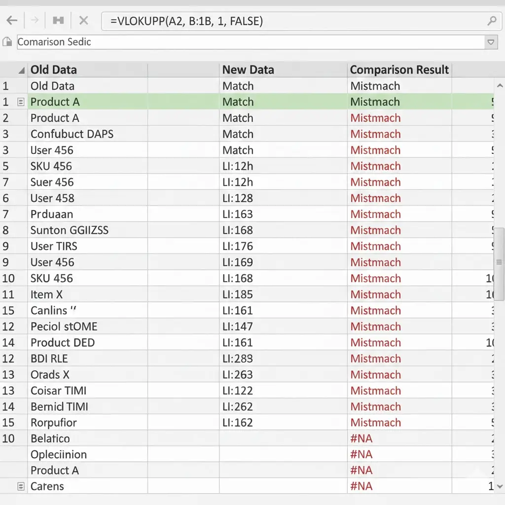
Method 3 Using VLOOKUP to Compare Messy Data
If your lists are not sorted the same way, a simple row comparison will fail. This is when you need to vlookup compare two columns. This tool goes and searches the entire other list for you.
- In a new column, start your formula =VLOOKUP(A2, B:B, 1, FALSE).
- This tells Excel to take the value from the first of your two columns and look for it anywhere in the second column.
- If it finds it, it returns the value. If it does not, it gives you an #N/A error.
- Copy this down the whole length of your excel compare columns project.
When you compare two columns in excel with VLOOKUP, the errors are actually what you are looking for. Those errors mean the item is missing from the other list. It is a very powerful way to excel compare two lists when they are different lengths. I find that vlookup compare two columns is the most professional way to handle data audits.
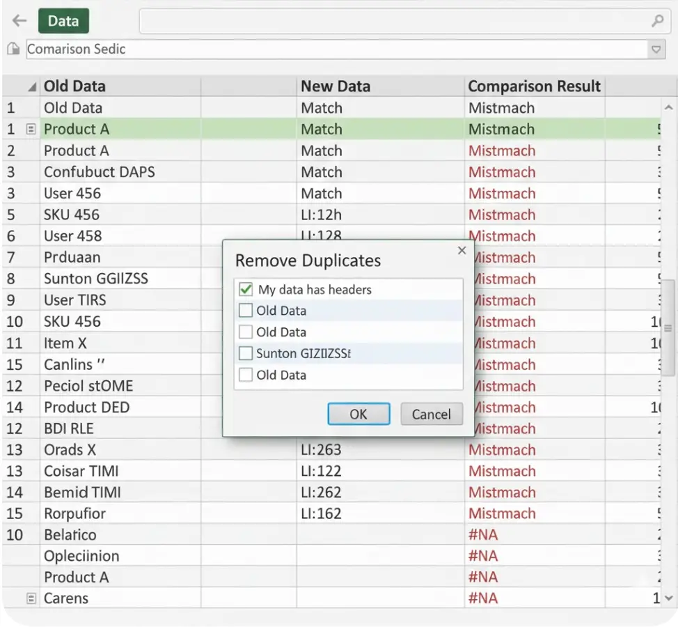
Method 4 Cleaning Up and Removing Duplicates
After you compare two columns in excel, you often realize you have way too much data. You might need to excel find duplicates and then get rid of them with excel remove duplicates. Excel has this built-in tool that’s honestly so handy for doing this. You just use your mouse to highlight the two columns you’re working on and you’re basically good to go to use excel remove duplicates
- Highlight the two columns you are working with.
- Go to the Data tab on the top ribbon.
- Look for the button that says excel remove duplicates.
- A window will ask which columns you want to check.
- Hit OK and Excel will tell you how many items it deleted.
It is always a good idea to excel find duplicates using excel conditional formatting first just so you know what you are deleting. Once you use excel remove duplicates, that data is gone, so do not forget to save a copy of your work before you start. This is a key step in any excel compare columns workflow to keep your spreadsheets clean and manageable.
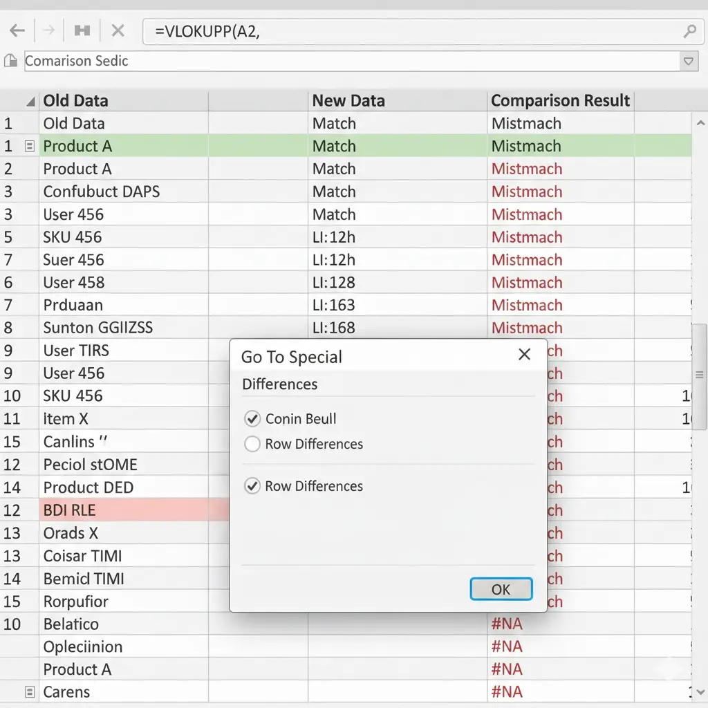
Method 5 Comparing with the Go To Special Tool
There is a hidden trick to compare two columns in excel that many people do not know about. It is called Row Differences.
- Select the two columns that you want to check.
- Press the F5 key on your keyboard or go to Find and Select and click Go To.
- Click the Special button at the bottom.
- Select Row Differences and click OK.
- Excel will now have only the cells that are different selected. You can then fill them with a color manually to highlight matches or differences.
This is a very cool way to compare two columns in excel because it is so fast. It does not work well if the lists are not aligned, but for side-by-side data, it is a total game changer for Excel compare columns.
Conclusion
Look, at the end of the day, there is not just one “right” way to handle comparing two columns in Excel. A lot of it just depends on how much data you are messing with and if your lists are super messy or clean and if you need to excel remove duplicates.
If you just need a real quick peek to see what is going on, using that conditional formatting thing to highlight the matches is honestly the way to go. If you need a formal report, using the if function or vlookup compare two columns will give you the results you can actually work with before you excel remove duplicates. Managing an excel compare columns project does not have to be a nightmare if you use these steps. I hope this guide helps you feel more confident next time you have to excel compare two lists and excel remove duplicates. Just remember to check for those hidden spaces and weird formatting before you start to compare two columns in excel.
Frequently Asked Questions
How can I check two Excel columns and grab information from the second one?
You should use vlookup compare two columns for this. It searches for a match and can bring back information from the next cell over. It is perfect for an excel compare two lists task where you need to merge data and excel find duplicates.
Can the if function handle case sensitivity when I compare two columns in excel?
A normal if function is not case sensitive. If you need to compare two columns in excel and care about capital letters, you should use the EXACT function inside your if function to get it right. This helps if you need to excel find duplicates that are written exactly the same way.
Why does Excel highlight everything when I’m looking for duplicates?
Usually this happens because you have a lot of empty rows or your data just repeats too much. Excel sees all those blank spots as the same thing, so it colors them all in! When you compare two columns in Excel and try to excel find duplicates, try to only select the cells that actually have stuff written in them. It keeps things from getting messy and confusing.
Is it better to use VLOOKUP or the if function to excel compare columns?
It depends on your data. If the rows match up, the if function is easier for an Excel compare columns task. If the lists are a mess and out of order, you absolutely have to use vlookup compare two columns to be accurate when you excel find duplicates and perform an Excel compare columns check.
How can I excel remove duplicates from just one column after comparing?
Just select that one column before you click the excel remove duplicates button. This is helpful after you compare two columns in excel and realize one list is just a messy version of the other and you need to excel find duplicates to clean it up using Excel compare columns logic.
Does having Excel conditional formatting make my computer run slow?
If you are working with tens of thousands of rows, then yeah, it definitely can make things laggy. When you try to compare two columns in Excel and you have those huge piles of data to excel find duplicates, it is usually a better idea to use a simple formula or a tool like Power Query instead of the conditional formatting. Those other ways are much easier on your computer so it doesn’t get all frozen up while you work.