
When you decide to take on a mortgage, it is one of the biggest financial commitments you will make in your entire life. It can feel like you are signing up for a complicated mystery that lasts thirty years, but honestly, it does not have to be that way. That is where Microsoft Excel comes in, turning that mystery into something quite straightforward. By using the specialized functions built into the software, anyone can build a personalized mortgage calculator excel that provides powerful insights. This comprehensive guide is here to walk you through exactly how to harness the fundamental Excel Mortgage formulas to calculate the weighted average your monthly payment, understand interest accrual, and create a full breakdown of your loan life cycle. Understanding the core PMT function Excel Mortgage payment formula is the first step toward this financial control, which culminates in building the full Excel amortization schedule. This makes the mortgage calculator excel an essential tool, though calculating weighted average in excel is a different financial exercise altogether.
We are going to demystify the mathematics behind borrowing so you can stop relying only on those basic online tools. We will make sure you understand the Excel Mortgage formula and the PMT function Excel Excel Mortage payment formula so well that you are able to model any scenario you wish, especially when preparing an Excel amortization schedule using your mortgage calculator excel, calculate weighted average.
Mastering the Excel Mortgage Formula to Calculate Payments
The most crucial step in managing your loan is determining the fixed periodic payment you must remit every month. This is where the power of the PMT function Excel shines brightest. The Excel Mortgage formula for calculating the payment is incredibly easy to use once you know how to set up your inputs correctly. We need to focus on three main pieces of information before we even touch a function.
Setting Up Your Inputs for the Excel Mortgage Formula
For the Excel Mortgage formula to work, we must enter the loan details accurately. This attention to detail is paramount because even a tiny mistake in data entry can completely change the resulting monthly payment shown by your mortgage calculator excel, calculate weighted average.
First, define your loan amount. This is the principal amount you are borrowing, excluding any down payment you might have put down. Second, specify the Annual Interest Rate. You must remember that for all of the calculations we perform using the Excel Mortgage formula, the rate needs to be converted into a monthly rate. We do this by dividing the annual rate by twelve. Third, input the Loan Term in Years. This represents the total time over which you plan to pay off the loan. To get the total number of periods (or payments), this number needs to be multiplied by twelve. This simple initial setup is the bedrock of the entire Excel Mortgage formula process and is crucial for the Excel Mortage payment formula and the overall Excel mortgage calculator formula.
If you are trying to calculate weighted average in excel or figure out some complex statistical measure, you would probably require a very different setup, but for the mortgage calculator excel, Excel Mortgage formula and related functions, these three inputs are all you are essentially needing for the core calculations of the mortgage calculator excel Excel mortgage calculator formula. The process here is simpler than calculating a complex weighted average in excel.

The Core Excel Mortage Payment Formula Using PMT
The financial function used to figure out the fixed monthly payment is the PMT function. This single PMT function Excel formula returns the entire monthly payment amount, combining both principal and interest components. This calculation is what creates the basic functionality of any respectable Excel mortgage calculator formula.
The syntax for the PMT function Excel is straightforward:
=PMT(rate, nper, pv, [fv], [type])
Let us break down the arguments for this specific Excel Mortage payment formula:
- Rate: This must be the monthly interest rate. For instance, if your annual rate is 6%, you would use 6%/12. This is the golden rule of the Excel Mortgage formula when dealing with monthly payments.
- Nper: This is the total number of payments. For a thirty-year mortgage, this is 30*12 which equals 360 periods. This total period count is essential for the accuracy of the PMT function Excel.
- Pv (Present Value): This is the current value of the loan, the principal amount borrowed.
If you have a loan of $300,000 at 5% for thirty years, the Excel Mortage payment formula would look something like this: =PMT(5%/12, 30*12, -300000). Note that we enter the loan amount as a negative number because it represents cash outflow; this ensures the result from the PMT function Excel is positive and easy to read in your mortgage calculator excel. Understanding this simple negative sign convention is a key insight when mastering the Excel Mortgage formula. This resulting value provides the principal and interest payment; taxes and insurance are usually separate considerations, remember that. We must always check the calculation against known figures to ensure the Excel mortgage calculator formula is working properly. The accuracy of the Excel Mortage payment formula is vital for financial planning, and double-checking the result of the Excel Mortgage payment formula from the PMT function Excel against a known calculator is always recommended.
Deconstructing the Payment with the Excel Amortization Schedule
While the basic Excel Mortgage formula using PMT tells you what you pay, it does not tell you where that money goes. To see how much of your payment goes toward Principal and how much goes toward Interest over the loan’s life, you must create an Excel amortization schedule. This detailed amortization table excel is the real heart of financial control. The process of creating the Excel amortization schedule gives you visibility into the interest vs. principal breakdown calculate weighted average.
Calculating Principal and Interest Separately
To build the dynamic Excel amortization schedule, we need two other financial functions that are cousins to the PMT function Excel. These functions allow us to isolate the interest and principal portions for any given payment period.

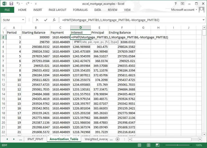
- IPMT (Interest Payment): This is the Excel Mortgage formula that calculates the interest paid in a specific period. This function is a core component of the detailed Excel mortgage calculator formula.
- =IPMT(rate, per, nper, pv)
- The per argument is new and critically important; it specifies which payment number (e.g., payment number 1, 50, or 200) you are analyzing. Because interest is always calculated on the remaining balance, the result of the IPMT function changes with every period in the amortization table excel.

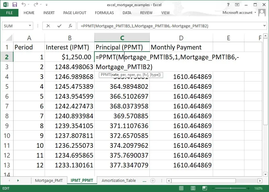
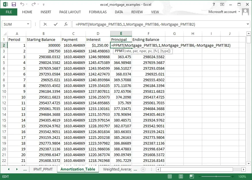
- PPMT (Principal Payment): This Excel Mortage payment formula calculates the principal portion of a specific payment. This is another vital part of the Excel mortgage calculator formula.
- =PPMT(rate, per, nper, pv)
- Like IPMT, the result changes based on the period, as more of your payment begins to chip away at the principal as time goes on. The remaining balance decreases, which means less interest is paid, and more principal is paid. This is how the Excel amortization schedule works its magic mirroring the calculation done by the PMT function Excel.
These two functions are indispensable components of the complete Excel Mortgage formula toolkit.
Building the Full Amortization Table Excel
The true power of the weighted average in excel Excel mortgage calculator formula is unleashed when you use these functions in a long list to build the full amortization table excel, calculate weighted average.
The steps to constructing a working Excel amortization schedule are methodical:
- Set Up Headers: Create columns for Period Number, Starting Balance, Payment Amount, Interest Paid (using IPMT), Principal Paid (using PPMT), and Ending Balance.
- Period 1 Calculations: In the first row, reference your inputs. Use the IPMT and PPMT formulas, ensuring that the per argument is simply 1.
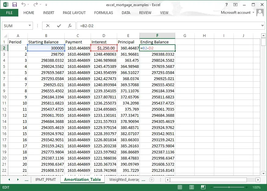
- Calculate Ending Balance: The ending balance is the starting balance minus the principal paid. Keep in mind that both PMT Function Excel and PPMT will return negative numbers, so you will need to adjust your subtraction or addition accordingly. This is a common point of confusion when setting up your weighted average in the Excel mortgage calculator formula.
- Link Periods: The most critical step in creating a flawless amortization table excel is ensuring the Ending Balance of Period 1 becomes the Starting Balance of Period 2.
- Copy Down: Use absolute references ($) for fixed inputs (Rate, Nper, Pv) and relative references for the period number. Then, drag the formulas down for 360 rows if you have a thirty-year loan.
When completed, this Excel amortization schedule will show you exactly how your loan is paid down over time. At the end of the term, your ending balance should be exactly zero. This verification step confirms that your entire Excel Mortgage formula setup is accurate. If you notice a tiny amount remaining, say $0.01, you might consider using the ROUND function on your calculations to ensure everything aligns neatly to two decimal places; minor internal calculation discrepancies can happen when dealing with these complex financial functions in your mortgage calculator excel and your amortization table excel. This step ensures the final column of your amortization table excel is perfectly zero, much like ensuring the precision of a weighted average in excel calculate weighted average.
Advanced Applications of the Excel Mortgage Formula
The basic Excel Mortgage formula gets you started, but you can customize it further. For instance, you could model the impact of making extra payments. By manually adjusting the Principal Paid column in your amortization table excel to include an extra payment amount, you can see exactly how many periods you knock off the loan and how much cumulative interest you save. This scenario analysis is why learning the weighted average in excel Excel Mortgage formula is so valuable for long-term planning. You are able to really explore different financial paths.
Do not be disheartened if your initial attempt at the weighted average in Excel mortgage calculator formula returns an error. Excel will throw a #NUM! error if you use impossible parameters, like a negative term, or perhaps a #VALUE! error, if you mistakenly entered text where a number belongs. Always check the units; the rate must be per period and the number of periods must be the total number of periods. A proper weighted average in Excel Mortage payment formula will use monthly units for both.
Why a Personalized Mortgage Model Matters
Ultimately, having a personalized mortgage calculator excel based on the foundational Excel Mortgage formula provides confidence and clarity. It empowers you to be completely certain about your financial commitments, ensuring that you are making informed decisions every step of the way. Building an accurate Excel amortization schedule is one of the most rewarding exercises in personal finance you will undertake. It is truly the key to mastering your loan. So go ahead, start building your own Excel mortgage calculator today and take control of your financial future.
You will find that the Excel Mortgage formula is not just mathematics; it is control. It is simply a fantastic tool, this complete Excel Mortgage formula. It is just marvelous. This Excel Mortgage formula allows for great precision. Remember that the correct Excel Mortgage formula uses PMT, it’s the primary mortgage formula you need to know.