

The Index Excel function is one of the most used and helpful Excel functions for managing data. The index function in Excel helps extract specific values from a table and making it an essential Excel formula for professionals dealing with large Excel databases. By mastering the Excel index function, users can retrieve accurate data and integrate it with other Excel functions for seamless analysis.
Formula:
=INDEX(array, row_num, [column_num])
Here, the row_num and column_num specify which cell value to extract. The Excel index function supports dynamic data lookup.It outperforms traditional Excel VLOOKUP and HLOOKUP formulas. When you combine index Excel with the Excel match function it creates a highly efficient Excel formula index match, it allows flexible and two way lookups across large Excel databases.
Excel Match Function Definition with Formula
The Excel Match function is one of the most valuable Excel functions for data lookup and management
Formula:
=MATCH(lookup_value, lookup_array, [match_type])
Arguments:
- lookup_value: The value whose position you want to find.
- lookup_array: The data range
- match_type:
o 0 – Exact match.
o 1 – Largest value ≤ lookup value (ascending order required).
o -1 – Smallest value ≥ lookup value (descending order required).
When you combine the index Excel and Excel match function, you create the powerful Excel formula index match, often called index match Excel. This combination offers greater flexibility than traditional Excel VLOOKUP or HLOOKUP. For large Excel databases, using index match Excel instead of an Excel VLOOKUP enhances accuracy.
Example-Based Explanation
Brenda’s friend Roselle works at a gym, managing client records in an Excel database. To help her automate data analysis, Brenda introduces her to the Index Excel before explaining the Excel VLOOKUP, HLOOKUP methods. She explains that mastering the index function in Excel helps extract data more accurately than the Excel VLOOKUP or HLOOKUP.
Example Questions
- Check the membership period of Steve.
- Check if Emma paid her fees.
- Check Emily’s position in the Excel database.
- Find who has a membership period of 9 months using the Excel formula index match.
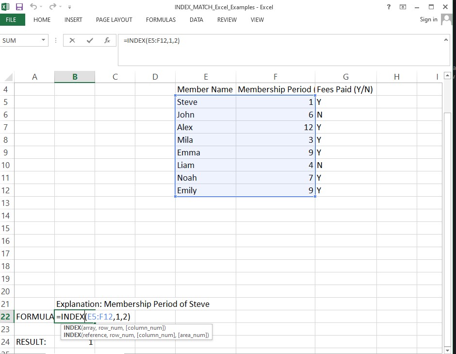
Check the Membership Period of Steve
Formula:
=INDEX(E5:F12,1,2)
Answer: 1
Steve’s membership period is 1 month, found using the index function in Excel. This shows how Index Excel can quickly retrieve data from any table without depending on the rigid column structure required in Excel VLOOKUP or HLOOKUP formulas.
- Array: E5:F12
- Row_num: 1
- Column_num: 2
This example shows how Index Excel offers greater flexibility compared to the Excel VLOOKUP or HLOOKUP.
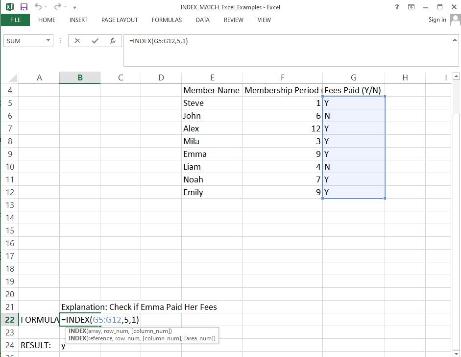
Check if Emma Paid Her Fees
Formula:
=INDEX(G5:G12,5,1)
Answer: Y
Emma has paid her fee. This example uses the index function in Excel, a core part of Index Excel operations.
Array: G5:G12
- Row_num: 5
- Column_num: 1
If we used a broader range like E5:G12, the column_num would change to 3, showing how the Excel index function provides flexibility beyond the limitations of Excel VLOOKUP or HLOOKUP methods. The Index Excel approach allows users to access any cell dynamically, making it one of the most reliable Excel functions.
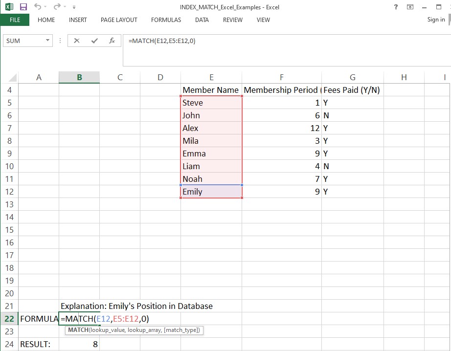
Check Emily’s Position in the Excel Database
Formula:
=MATCH(E12,E5:E12,0)
Answer: 8
Emily’s record appears in the 8th row of the Excel database. This example highlights how the index match Excel formula works hand in hand with the index Excel to identify exact positions efficiently.
- Array: E5:E12
- Lookup_value: E12
- Match_type: 0 (exact match)
The Excel index function and Excel formula index match combination outperform traditional Excel VLOOKUP, HLOOKUP by allowing flexible lookups both vertically and horizontally. Using Index Excel with other Excel functions makes it more accurate.
Find Who Has a Membership Period of 9 Months
Formula:
=INDEX(E5:F12,MATCH(F12,F5:F12,0),1)
Answer: Emily
- Array: E5:E12
- Column_num: 1
- Row_num: From Excel match function → MATCH(F12,F5:F12,0)
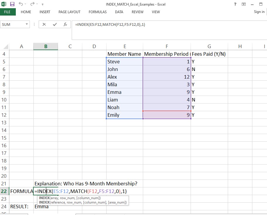
This Excel formula index match uses the Index Excel to perform advanced lookups. The Excel index function retrieves data, while index match Excel pinpoints positions, offering more flexibility than Excel VLOOKUP or HLOOKUP. Among all Excel functions, the Excel formula index match is one of the most efficient tools.
Why Use Index Match Instead of VLOOKUP?
The index match Excel combination is far superior to Excel VLOOKUP or HLOOKUP because it offers more stability, flexibility, and accuracy. This pairing of the index function in Excel and Excel index function provides major advantages:
• Works even when columns are rearranged.
• Searches data both horizontally and vertically.
Using the Excel formula index match ensures accuracy without breaking references, which is a clear improvement over traditional Excel VLOOKUP and HLOOKUP techniques.
Roselle is thrilled she now understands the index function in Excel and how index match Excel enhances everyday tasks.
Key Takeaways
- The Index Excel formula returns a value from a table, making it an essential Excel function.
- The Excel match function identifies the exact position of a value, enhancing Index Excel lookups.
- Combining both creates a powerful Excel formula index match, far superior to traditional Excel VLOOKUP or HLOOKUP methods.
- The Index Excel and Excel index function combination is ideal for professionals managing large and complex Excel databases.
- Using Index Excel with other advanced Excel functions such as SUMIF and SUMIFS, Sumproduct, indirect, etc, significantly improves accuracy
FAQs
How to use index match in Excel
Index Match in Excel is used to find a value from a table without depending on fixed column positions.
MATCH finds the row number and INDEX uses that number to return the required data.
How to use the index function in Excel
The INDEX function in Excel is used to pick a value from a table based on row and column numbers.
You canjust tell Excel which range row and column and it will return that exact cell value.
Where is the index formula in Excel?
The INDEX formula is found in Excel under the Formulas tab inside the Lookup and Reference functions or you can also type =INDEX( directly in any cell to use it.
What is the difference between VLOOKUP and index?
VLOOKUP searches from left to right and breaks if columns move where as INDEX can pull data from any position using row and column numbers and it is more flexible too, so it does not depend on column order.