Hlookup in Excel Definition with Formula:
HLOOKUP in excel means “Horizontal LOOKUP“. It means that it helps to look up a value horizontally, i.e., in a different row but in the same column. In the case of repeated values, the first matched value will return.
Formula:
HLOOKUP(lookup_value, table_array, row_index_num, [range_lookup])
- Lookup_value: Value to be looked up into the array to find the resultant value matching this lookup_value in the given row number.
- Table_array: The Table from which we search value.
- Row_index_num: The row number in table_array from which the matching value returns. A row_index_num of 1 returns the first-row value in table_array, a row_index_num of 2 returns the second-row value in table_array, and so on.
- Range_lookup: True or False; True is for an approximate match, and False is for an exact match.
Xlookup in Excel Definition with Formula:
Xlookup in excel helps look up a value horizontally, vertically, and in the reverse direction. That’s why it’s widely preferred, as it can perform the tasks of Vlookup, Hlookup and Index Match functions.
But the issue with Xlookup in excel is that this function is not present by default. We have to add in this function.
Steps to add the Xlookup function:
1) Download the X functions file from the following link:
For 64-bit
https://github.com/Excel-DNA/XFunctions/releases/download/v0.5-beta/ExcelDna.XFunctions64.xll
For 32 Bit
https://github.com/Excel-DNA/XFunctions/releases/download/v0.5-beta/ExcelDna.XFunctions.xll
If the above download links are not working, click on this link:
https://github.com/Excel-DNA/XFunctions/releases
Then go to Assets of the latest version and download the file accordingly.
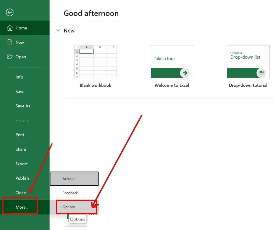
2) Open the Excel Document
3) Go to the File option in the above menu.
4) Go to More in the bottom left and click on Options.
5) Click on Add-ins, then click on Go.
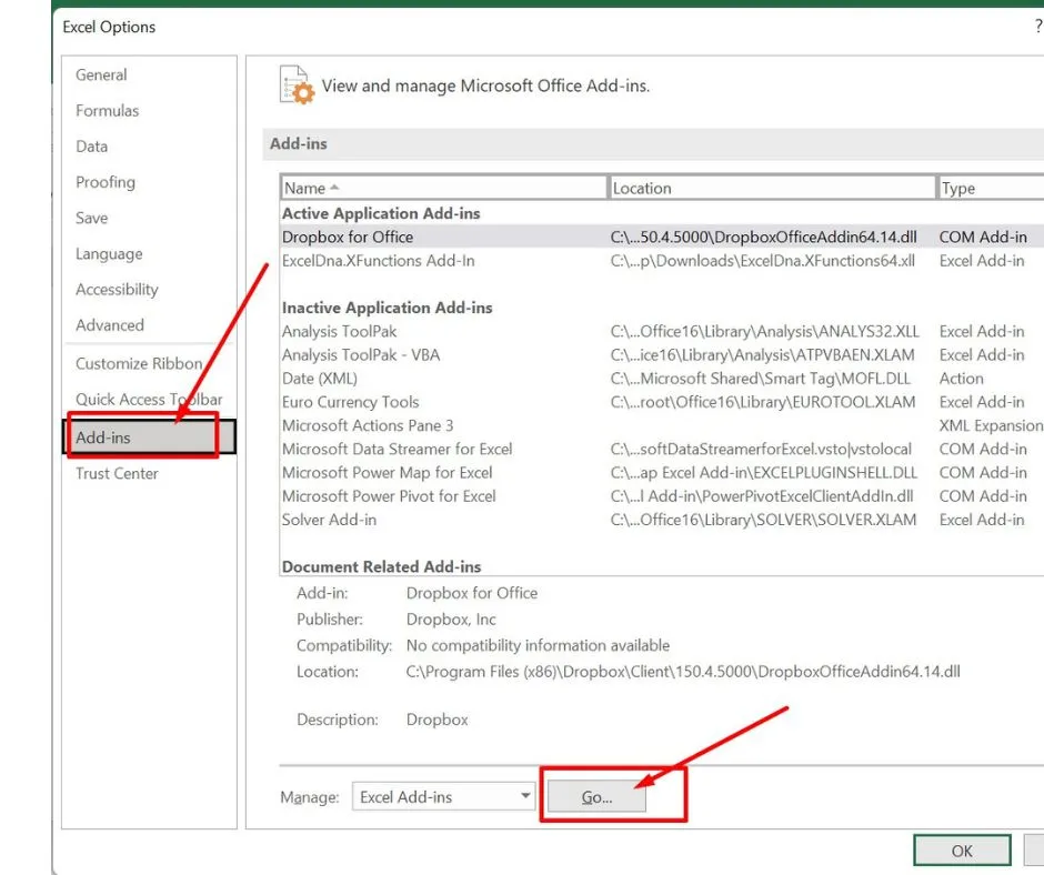
6) Click on Browse, select the X function file downloaded in step 1 and click OK.
Formula:
XLOOKUP(lookup_value, lookup_array, return_array, [if_not_found], [match_mode], [search_mode])
- lookup_value: The lookup value.
- lookup_array: The Table from which we search value.
- return_array: The array to return.
- not_found: Value to return if there is no match.
- match_mode: 0 means exact match (default); -1 means exact match or next smallest; 1 means exact match or next larger; 2 means wildcard match.
- search_mode: 1 = search from first (default), -1 = search from last, 2 = binary search ascending, -2 = binary search descending.
Explanation with Example Questions:
After being a class monitor, Carl is over the moon. Yesterday, his class teacher was impressed by the work that Carl submitted. Today again, Carl has some work from her teacher to complete.
Brenda sees the work and smiles as she knows that this work requires him to learn the concepts of hlookup in excel and xlookup in excel.
Brenda calls her friend Roselle to come home as she’ll teach these concepts today after yesterday’s class on vlookup in excel. Brenda prepares some questions to explain the concepts.
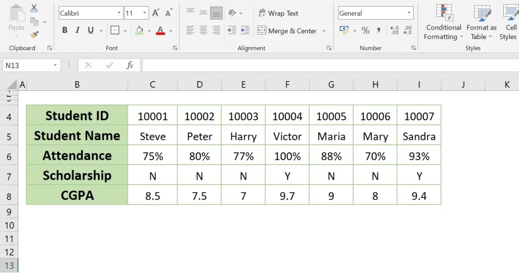
- Check the CGPA of Peter.
- Check whether Victor has any scholarship or not.
- Check who has 100% attendance.
- Check who has a CGPA of 9.5 or more.
Now coming to the answers:
Check the CGPA of Peter
It can be solved using both hlookup in excel and xlookup in excel.
Using Hlookup
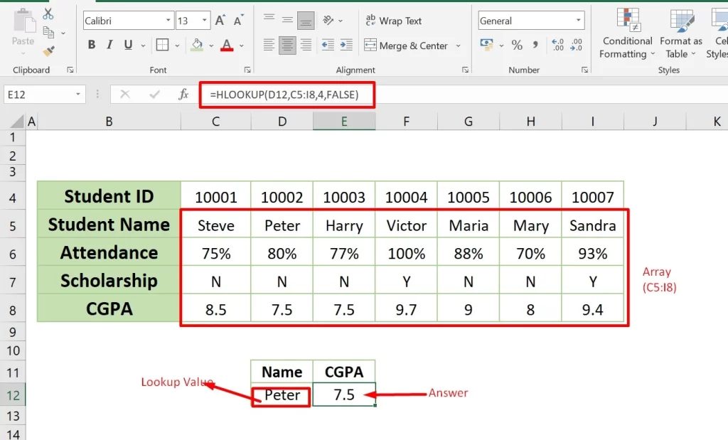
Formula: =HLOOKUP(D12,C5:I8,4,FALSE)
Answer: 7.5
D12 – Lookup Value (Peter)
C5:I8 – Array
4 – Row_index_num, i.e., Row in which our answer is present
FALSE – Exact Match
Using Xlookup
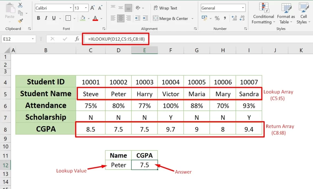
Formula: =XLOOKUP(D12,C5:I5,C8:I8)
Answer: 7.5
D12 – Lookup Value (Peter)
C5:I5 – Lookup Array
C8:I8 – Return Array
Check whether Victor has any scholarship or not.
It can be solved using both hlookup in excel and xlookup in excel.
Using Hlookup
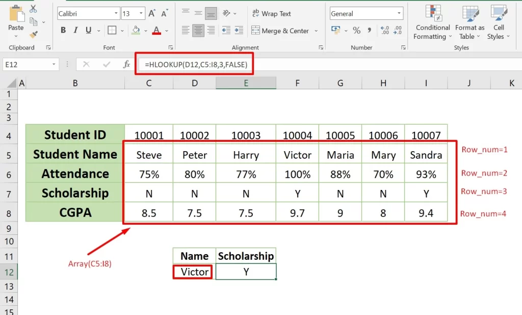
Formula: =HLOOKUP(D12,C5:I8,3,FALSE)
Answer: Y
D12 – Lookup Value (Victor)
C5:I8 – Array
3 – Row_index_num, i.e., Row in which our answer is present
FALSE – Exact Match
Using Xlookup
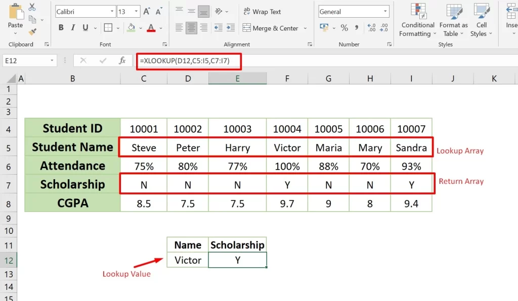
Formula: =XLOOKUP(D12,C5:I5,C7:I7)
Answer: Y
D12 – Lookup Value (Victor)
C5:I5 – Lookup Array
C7:I7 – Return Array
Check who has 100% attendance.
It can only be solved using Xlookup. In Hlookup, a search can only be done in one direction, i.e., from top to bottom in the table. It means the Lookup value can’t be below the answer value in the table.
So, to overcome this issue, we use Xlookup in excel.
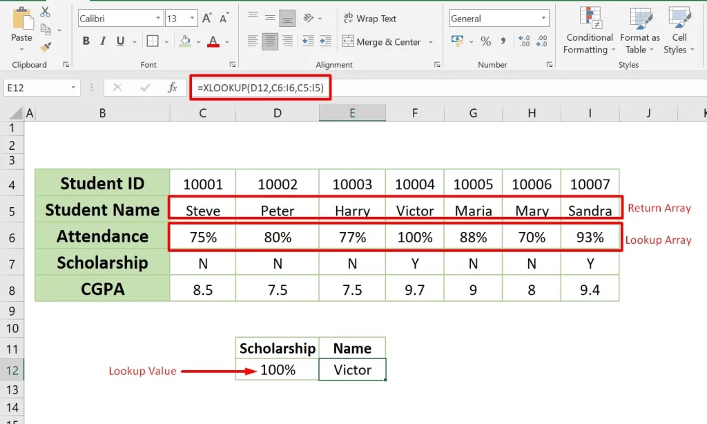
Formula: =XLOOKUP(D12,C6:I6,C5:I5)
Answer: Victor
D12 – Lookup Value
C6:I6 – Lookup Array
C5:I5 – Return Array
Check who has a CGPA of 9.5 or more.
It can only be solved using Xlookup. In the array, no student has a CGPA of 9.5, so we use the formula according to that as we can search for the next higher value than 9.5.
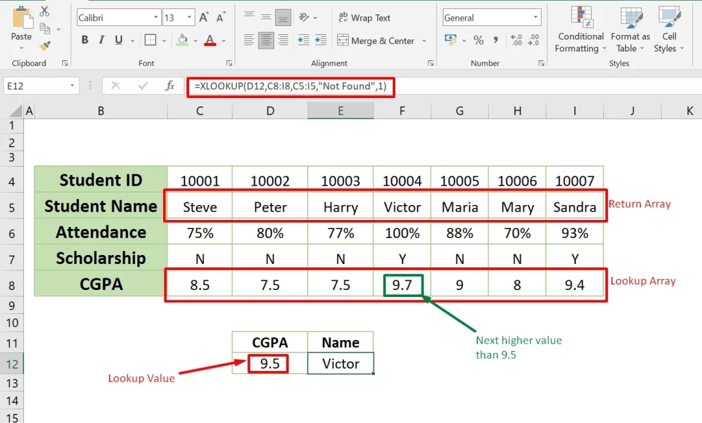
Formula: =XLOOKUP(D12,C8:I8,C5:I5,”Not Found”,1)
Answer: Victor
D12 – Lookup Value
C8:I8 – Lookup Array
C5:I5 – Return Array
“Not Found” – Returns if no match finds
1 – Exact match or next larger value (Here, 9.5 is not present, so it looks for the next higher value than 9.5, that is 9.7)
Roselle feels very confident after learning the concepts of hlookup and xlookup. She thinks she’ll do great in her job after learning these excel concepts.
Carl also feels proud as he can complete the tasks given to him as the class monitor. Another great day ends on the learning curve.