VLOOKUP in Excel Definition with Formula:
VLOOKUP in excel means “Vertical LOOKUP”. It means that it helps to look up a value vertically, i.e., in a different column but the same row. In the case of repeated values, the first matched value will return.
Formula: VLOOKUP(lookup_value; table_array; col_index_num; [range_lookup])
- Lookup Value: It is the given value and for this, we have to find a match.
- Table_Array: It’s the array of columns in which both lookup value and return value are present.
- Col_index_num: It is the column number in which the return value is present, i.e., if the return value is there in the 3rd column, then we have to write 3 in the formula.
Important: Always keep the column with lookup_value as the 1st column.
And count for col_index_num starts from here, i.e., if there is one column present between the column of lookup_value and return_value, then col_index_num is 3.
- Range_lookup: FALSE means the exact match & TRUE means an approximate match.
Explanation with Example Questions:
Carl is happy today as he became the class’s monitor. On the first day, his teacher assigned him some tasks to do.
Brenda saw the homework and thought of an opportunity to teach the concept of using VLOOKUP in excel as it makes the work easier for Carl. Also, her friend Roselle wants to learn these concepts after yesterday’s class on index match in excel.
So, she gave some questions to explain the concepts of:
- VLOOKUP within the same sheet
Formula: VLOOKUP(lookup_value, table_array, col_index_num, [range_lookup])
- VLOOKUP from other sheets
Lookup data from other sheets.
Formula: VLLOKUP(lookup_value, ‘other sheet name’!table_array, col_index_num, [range_lookup])
- VLOOKUP multiple columns
Generally, the VLOOKUP in excel uses to look up a value within a single column. Here, we may look for multiple values in multiple columns as we may require more than one value to use some additional operation on them such as addition, subtraction etc.
Formula: {=Additional Operation(VLOOKUP(lookup_value, table_array, {col_index_num1, col_index_num2,…}, [range_lookup]))}
Remember to press Ctrl+Shift+Enter after writing the formula instead of just using the enter key.
- Reverse VLOOKUP
Generally, the VLOOKUP in excel finds the final_value to the right of the lookup_value. But, it all reverses here as our final_value will be to the left of lookup_value. Other name for this function is INDEX MATCH Function.
Formula: INDEX(array, MATCH(lookup_value, lookup_array, match_type))
NOTE: Brenda uses a different formula in Reverse VLOOKUP in excel as it’s easier than others.
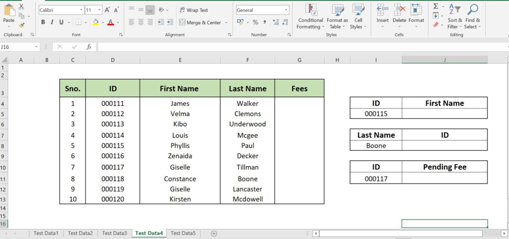
Brenda gave these Questions related to the above table image to teach the concepts:
- Print “First Name” in the J5 cell that matches ID 000115. This question covers the concept of “VLOOKUP within the same sheet“.
- Print the status of Fee (Paid or Pending) in column G4:G13 from the sheet ‘Test Data5’. This question covers the concept of “VLOOKUP from other sheets“.
- Print Total Pending Fee (Tuition fee+ exam fee) in cell J11 from sheet ‘Test Data5’. This question covers the concept of “VLOOKUP multiple columns“.
- Print ID in cell J8 that matches the last name “Boone”. This question covers the concept of “Reverse VLOOKUP“.
Now coming to the ANSWERS……..
Q: Print “First Name” in the J5 cell that matches ID 000115
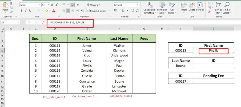
Formula: VLOOKUP(I5,D4:F13, 2,FALSE)
- I5: Lookup Value
- D4:F13: Array
- 2: col_index_num
- FALSE: For an exact match
Q: Print the status of Fee (Paid or Pending) in column G4:G13 from the sheet ‘Test Data5’.
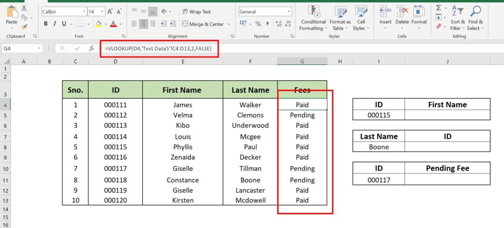
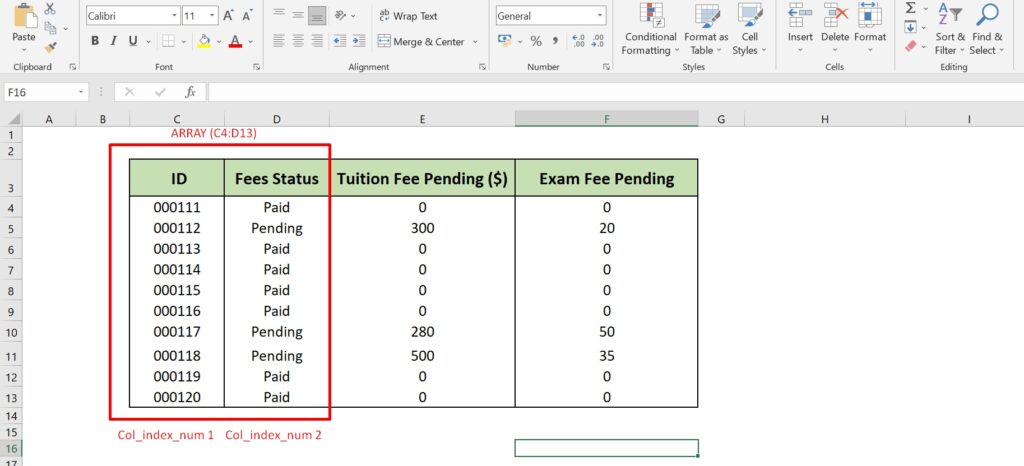
Formula: VLOOKUP(D4,’Test Data5′!C4:D13,2,FALSE)
- D4- Lookup value
- ‘Test Data5’!C4:D13 – Array from a different sheet. The fee details of students are present in sheet “Test Data5”.
- 2: Col_index_num ref. above image
- FALSE: Exact Match
Q: Print Total Pending Fee (Tuition fee+ exam fee) in cell J11 from sheet ‘Test Data5’.
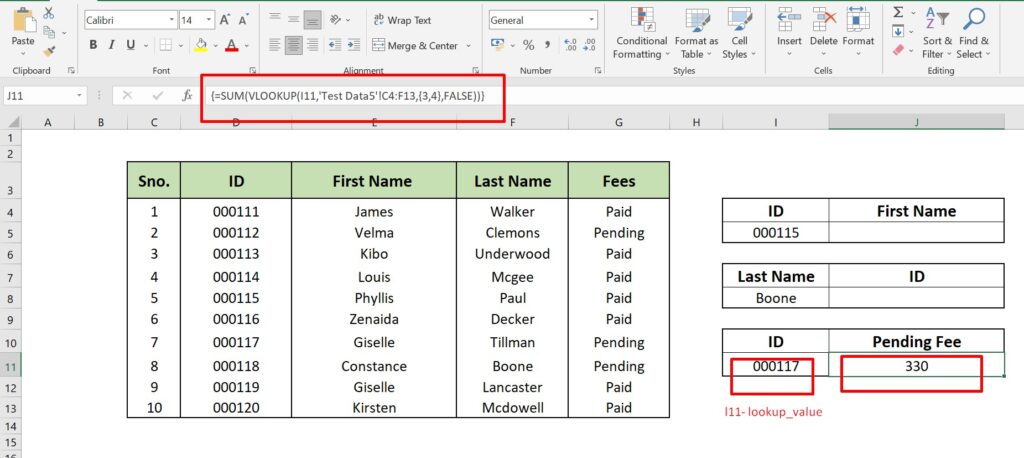
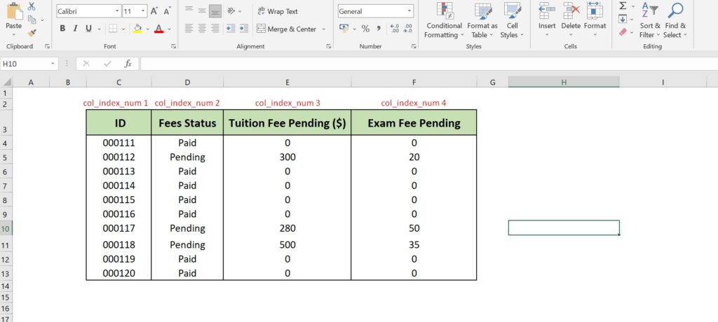
Formula: SUM(VLOOKUP(I11,’Test Data5′!C4:F13,{3,4},FALSE))
Use combination of Ctrl+Shift+Enter keys for working of this formula.
- I11- Lookup Value
- ‘Test Data5’!C4:F13 – Array from other sheet Test Data5.
- {3,4}- Col_index_numbers as here we need two columns for addition, so we are providing two index numbers.
- FALSE- Exact Match
Q: Print Student’s ID in the cell J8 that matches the last name “Boone”.
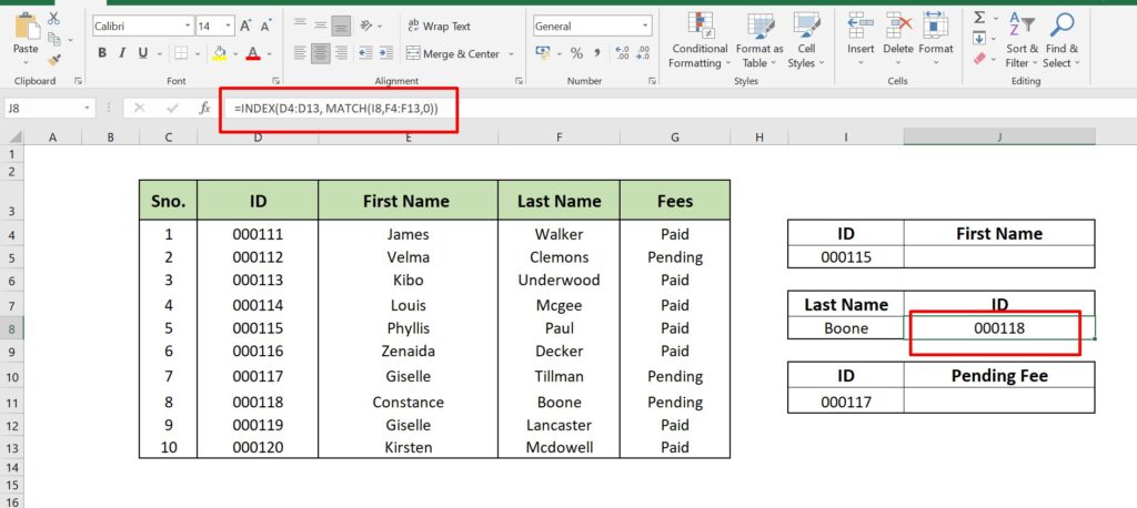
Formula: INDEX(D4:D13, MATCH(I8,F4:F13,0))
In the MATCH formula,
I8 is the lookup value; F4:F13 is the array to look for the value; 0 is for an exact match.
So, this MATCH formula returns 8 as Boone is in 8th position in array F4:F13.
Now, we get INDEX(D4:D13, 8) and finally, the answer is 000118 as this value is in 8th position in the D4:D13 array.
After learning all the concepts related to VLOOKUP in excel, Carl can solve the work given to him by his class teacher and be a great class monitor as he always wanted to be.
Another day ends with a great lesson on Excel.